Heap Sort

The binary heap data structures is an array that can be viewed as a complete binary tree. Each node of the binary tree corresponds to an element of the array. The array is completely filled on all levels except possibly lowest.
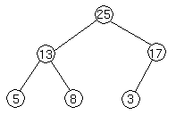
We represent heaps in level order, going from left to right. The array corresponding to the heap above is [25, 13, 17, 5, 8, 3].

The root of the tree A[1] and given index i of a node, the indices of its parent, left child and right child can be computed
 
PARENT (i)
        return floor(i/2)
LEFT (i)
        return 2i
RIGHT (i)
        return 2i + 1


Let's try these out on a heap to make sure we believe they are correct. Take this heap,
which is represented by the array [20, 14, 17, 8, 6, 9, 4, 1].

We'll go from the 20 to the 6 first. The index of the 20 is 1. To find the index of the left child, we calculate 1 * 2 = 2. This takes us (correctly) to the 14. Now, we go right, so we calculate 2 * 1 + 1 = 3. This takes us (again, correctly) to the 17.

Now let's try going from the 4 to the 20. 4's index is 7. We want to go to the parent, so we calculate 7 / 2 = 3, which takes us to the 17. Now, to get 17's parent, we calculate 3 / 2 = 1, which takes us to the 20.


Heap Property

In a heap, for every node i other than the root, the value of a node is greater than or equal (at most) to the value of its parent.

       
A[PARENT (i)] ≥A[i]

Thus, the largest element in a heap is stored at the root.


Following is an example of Heap:

By the definition of a heap, all the tree levels are completely filled except possibly for the lowest level, which is filled from the left up to a point. Clearly a heap of height h has the minimum number of elements when it has just one node at the lowest level. The levels above the lowest level form a complete binary tree of height h -1 and 2h -1 nodes. Hence the minimum number of nodes possible in a heap of height h is 2h. Clearly a heap of height h, has the maximum number of elements when its lowest level is completely filled. In this case the heap is a complete binary tree of height h and hence has 2h+1 -1 nodes.
Following is not a heap, because it only has the heap property - it is not a complete binary tree. Recall that to be complete, a binary tree has to fill up all of its levels with the possible exception of the last one, which must be filled in from the left side.


Height of a node

We define the height of a node in a tree to be a number of edges on the longest simple downward path from a node to a leaf.


Height of a tree

The number of edges on a simple downward path from a root to a leaf. Note that the height of a tree with n node is lg n which is (lgn). This implies that an n-element heap has height  lg n
In order to show this let the height of the n-element heap be h. From the bounds obtained on maximum and minimum number of elements in a heap, we get
2h ≤ n ≤ 2h+1-1
Where n is the number of elements in a heap.
2h ≤ n ≤ 2h+1
Taking logarithms to the base 2
h  ≤  lgn  ≤  h +1
It follows that h =  lgn.

We known from above that largest element resides in root, A[1]. The natural question to ask is where in a heap might the smallest element resides? Consider any path from root of the tree to a leaf. Because of the heap property, as we follow that path, the elements are either decreasing or staying the same. If it happens to be the case that all elements in the heap are distinct, then the above implies that the smallest is in a leaf of the tree. It could also be that an entire subtree of the heap is the smallest element or indeed that there is only one element in the heap, which in the smallest element, so the smallest element is everywhere. Note that anything below the smallest element must equal the smallest element, so in general, only entire subtrees of the heap can contain the smallest element.


Inserting Element in the Heap


Suppose we have a heap as follows

Let's suppose we want to add a node with key 15 to the heap. First, we add the node to the tree at the next spot available at the lowest level of the tree. This is to ensure that the tree remains complete.

Let's suppose we want to add a node with key 15 to the heap. First, we add the node to the tree at the next spot available at the lowest level of the tree. This is to ensure that the tree remains complete.


Now we do the same thing again, comparing the new node to its parent. Since 14 < 15, we have to do another swap:


Now we are done, because 15   20.

Four basic procedures on heap are
  1. Heapify, which runs in O(lg n) time.
  2. Build-Heap, which runs in linear time.
  3. Heap Sort, which runs in O(n lg n) time.
  4. Extract-Max, which runs in O(lg n) time.


Maintaining the Heap Property

Heapify is a procedure for manipulating heap data structures. It is given an array A and index i into the array. The subtree rooted at the children of A[i] are heap but node A[i] itself may possibly violate the heap property i.e., A[i] < A[2i] or A[i] < A[2i +1]. The procedure 'Heapify' manipulates the tree rooted at A[i] so it becomes a heap. In other words, 'Heapify' is let the value at A[i] "float down" in a heap so that subtree rooted at index i becomes a heap.

Outline of Procedure Heapify

Heapify picks the largest child key and compare it to the parent key. If parent key is larger than heapify quits, otherwise it swaps the parent key with the largest child key. So that the parent is now becomes larger than its children.
It is important to note that swap may destroy the heap property of the subtree rooted at the largest child node. If this is the case, Heapify calls itself again using largest child node as the new root.

Heapify (A, i)
  1. l ← left [i]
  2. r ← right [i]
  3. if l ≤ heap-size [A] and A[l] > A[i]
  4.     then largest ← l
  5.     else largest ← i
  6. if r ≤ heap-size [A] and A[i] > A[largest]
  7.     then largest ← r
  8. if largest  ≠ i
  9.     then exchange A[i] ↔ A[largest]
  10.         Heapify (A, largest)


Analysis

If we put a value at root that is less than every value in the left and right subtree, then 'Heapify' will be called recursively until leaf is reached. To make recursive calls traverse the longest path to a leaf, choose value that make 'Heapify' always recurse on the left child. It follows the left branch when left child is greater than or equal to the right child, so putting 0 at the root and 1 at all other nodes, for example, will accomplished this task. With such values 'Heapify' will called h times, where h is the heap height so its running time will be θ(h) (since each call does (1) work), which is (lgn). Since we have a case in which Heapify's running time (lg n), its worst-case running time is Ω(lgn).


Example of Heapify
 

Suppose we have a complete binary tree somewhere whose subtrees are heaps. In the following complete binary tree, the subtrees of 6 are heaps:


The Heapify procedure alters the heap so that the tree rooted at 6's position is a heap. Here's how it works. First, we look at the root of our tree and its two children.


We then determine which of the three nodes is the greatest. If it is the root, we are done, because we have a heap. If not, we exchange the appropriate child with the root, and continue recursively down the tree. In this case, we exchange 6 and 8, and continue.


Now, 7 is greater than 6, so we exchange them.


We are at the bottom of the tree, and can't continue, so we terminate.


Building a Heap

We can use the procedure 'Heapify' in a bottom-up fashion to convert an array A[1 . . n] into a heap. Since the elements in the subarray A[n/2+1 . . n] are all leaves, the procedure BUILD_HEAP goes through the remaining nodes of the tree and runs 'Heapify' on each one. The bottom-up order of processing node guarantees that the subtree rooted at children are heap before 'Heapify' is run at their parent.

BUILD_HEAP (A)
  1. heap-size (A) ← length [A]
  2. For i ←  floor(length[A]/2) down to 1 do
  3.         Heapify (A, i)

We can build a heap from an unordered array in linear time.


Heap Sort Algorithm

The heap sort combines the best of both merge sort and insertion sort. Like merge sort, the worst case time of heap sort is O(n log n) and like insertion sort, heap sort sorts in-place. The heap sort algorithm starts by using procedure BUILD-HEAP to build a heap on the input array A[1 . . n]. Since the maximum element of the array stored at the root A[1], it can be put into its correct final position by exchanging it with A[n] (the last element in A). If we now discard node n from the heap than the remaining elements can be made into heap. Note that the new element at the root may violate the heap property. All that is needed to restore the heap property.

HEAPSORT (A)
  1. BUILD_HEAP (A)
  2. for i ← length (A) down to 2 do
    exchange A[1] ↔ A[i]
    heap-size [A] ← heap-size [A] - 1
    Heapify (A, 1)

The HEAPSORT procedure takes time O(n lg n), since the call to BUILD_HEAP takes time O(n) and each of the n -1 calls to Heapify takes time O(lg n).


Now we show that there are at most én/2h+1ù nodes of height h in any n-element heap. We need two observations to show this. The first is  that if we consider the set of nodes of height h, they have the property that the subtree rooted at these nodes are disjoint. In other words, we cannot have two nodes of height h with one being an ancestor of the other. The second property is that all subtrees are complete binary trees except for one subtree. Let Xh be the number of nodes of height h. Since Xh-1 o ft hese subtrees are full, they each contain exactly 2h+1 -1 nodes. One of the height h subtrees may not  full, but contain at least 1 node at its lower level and has at least 2h nodes. The exact count is 1+2+4+ . . . + 2h+1 + 1 = 2h. The remaining nodes have height strictly more than h. To connect all subtrees rooted at node of height h., there must be exactly Xh -1 such nodes. The total of nodes is at least
(Xh-1)(2h+1 + 1) + 2h + Xh-1 which is at most n.
Simplifying gives
Xh ≤ n/2h+1 + 1/2.

In the conclusion, it is a property of binary trees that the number of nodes at any level is half of the total number of nodes up to that level. The number of leaves in a binary heap is equal to n/2, where n is the total number of nodes in the tree, is even and n/2 when n is odd. If these leaves are removed, the number of new leaves will be lg(n/2/2 or n/4. If  this process is continued for h levels the number of leaves at that level will be n/2h+1.


Implementation

void heapSort(int numbers[], int array_size)
{
int i, temp;

for (i = (array_size / 2)-1; i >= 0; i--)
siftDown(numbers, i, array_size);

for (i = array_size-1; i >= 1; i--)
{
temp = numbers[0];
numbers[0] = numbers[i];
numbers[i] = temp;
siftDown(numbers, 0, i-1);
}
}


void siftDown(int numbers[], int root, int bottom)
{
int done, maxChild, temp;

done = 0;
while ((root*2 <= bottom) && (!done))
{
if (root*2 == bottom)
maxChild = root * 2;
else if (numbers[root * 2] > numbers[root * 2 + 1])
maxChild = root * 2;
else
maxChild = root * 2 + 1;

if (numbers[root] < numbers[maxChild])
{
temp = numbers[root];
numbers[root] = numbers[maxChild];
numbers[maxChild] = temp;
root = maxChild;
}
else
done = 1;
}
}

Heap Sort

The binary heap data structures is an array that can be viewed as a complete binary tree. Each node of the binary tree corresponds to an element of the array. The array is completely filled on all levels except possibly lowest.

Hash Tables

Direct-address table

If the keys are drawn from the reasoning small universe U = {0, 1, . . . , m-1} of keys, a solution is to use a Table T[0, . m-1], indexed by keys. To represent the dynamic set, we use an array, or direct-address table, denoted by T[0 . . m-1], in which each slot corresponds to a key in the universe.

Following figure illustrates the approach.


Each key in the universe U i.e., Collection, corresponds to an index in the table T[0 . . m-1]. Using this approach, all three basic operations (dictionary operations) take θ(1) in the worst case.


Hash Tables

When the size of the universe is much larger the same approach (direct address table) could still work in principle, but the size of the table would make it impractical. A solution is to map the keys onto a small range, using a function called a hash function. The resulting data structure is called hash table.

With direct addressing, an element with key k is stored in slot k. With hashing =, this same element is stored in slot h(k); that is we use a hash function h to compute the slot from the key. Hash function maps the universe U of keys into the slot of a hash table T[0 . . .m-1].

h: U → {0, 1, . . ., m-1}

More formally, suppose we want to store a set of size n in a table of size m. The ratio α = n/m is called a load factor, that is, the average number of elements stored in a Table. Assume we have a hash function h that maps each key k U to an integer name h(k) [0 . . m-1]. The basic idea is to store key k in location T[h(k)].

Typical, hash functions generate "random looking" valves. For example, the following function usually works well

h(k) = k mod m             where m is a prime number.

Is there any point of the hash function? Yes, the point of the hash function is to reduce the range of array indices that need to be handled.


Collision(class between two numbers when the key is same)

As keys are inserted in the table, it is possible that two keys may hash to the same table slot. If the hash function distributes the elements uniformly over the table, the number of conclusions cannot be too large on the average, but the birthday paradox makes it very likely that there will be at least one collision, even for a lightly loaded table


A hash function h map the keys k and j to the same slot, so they collide.
There are two basic methods for handling collisions in a hash table: Chaining and Open addressing.


Collision Resolution by Chaining

Code
 When there is a collision (keys hash to the same slot), the incoming keys is stored in an overflow area and the corresponding record is appeared at the end of the linked list.


Each slot T[j] contains a linked list of all the keys whose hash value is j. For example, h(k1) = h(kn) and h(k5) = h(k2) = h(k7).


  • The worst case running time for insertion is O(1).


  • Deletion of an element x can be accomplished in O(1) time if the lists are doubly linked.


  • In the worst case behavior of chain-hashing, all n keys hash to the same

  • slot, creating a list of length n. The worst-case time for search is thus θ(n) plus the time to compute the hash function.
    keys: 5, 28, 19, 15, 20, 33, 12, 17, 10
    slots: 9
    hash function = h(k) = k mod 9
    h(5)   =    5 mod 9 = 4
    h(28) =  28 mod 9 = 1
    h(19) = 19 mod  9 = 1
    h(15) =  15 mod 9 = 6
    h(20) =  20 mod 9 = 2
    h(33) =  33 mod 9 = 6
    h(12) =  12mod  9 =  3
    h(17) =  17 mod 9 = 8
    h(10) =  10 mod 9 = 1

    Figure
    A good hash function satisfies the assumption of simple uniform hashing, each element is equally likely to hash into any of the m slots, independently of where any other element has hash to. But usually it is not possible to check this condition because one rarely knows the probability distribution according to which the keys are drawn.

    In practice, we use heuristic techniques to create a hash function that perform well. One good approach is to derive the hash value in a way that is expected to be independent of any patterns that might exist in the data (division method).

    Most hash function assume that the universe of keys is the set of natural numbers. Thus, its keys are not natural to interpret than as natural numbers.


    Method for Creating Hash Function

    1. The division method.
    2. The multiplication method.
    3. Universal hashing.


    1. The Division Method
    Map a key k into one of m slots by taking the remainder of k divided by m. That is, the hash function is
    h(k) = k mod m.

    Example:
        If table size m = 12
                    key k = 100
        than
            h(100) = 100 mod 12
                       = 4

    Poor choices of m


    m should not be a power of 2, since if m = 2p, then h(k) is just the p lowest-order bits of k.
    So, 2p may be a poor choice, because permuting the characters of k does not change value.


    Good m choice of m


    A prime not too close to an exact of 2.


    2. The Multiplication Method

    Two step process


    Step 1:
    Multiply the key k by a constant 0< A < 1 and extract the fraction part of kA.
    Step 2:
    Multiply kA by m and take the floor of the result.
     
     
    The hash function using multiplication method is:
    h(k) = [m(kA mod 1)] 
    where "kA mod 1" means the fractional part of kA, that is, kA - [ kA ]

    Advantage of this method is that the value of m is not critical and can be implemented on most computers.
    A reasonable value of constant A is
     
    A~= (sqrt5 - 1) /2=0.618033....

    3. Universal Hashing
     This involves choosing a hash function randomly in a way that is independent of the keys that are actually going to be stored. We select the hash function at random from a carefully designed class of functions.


    Let table size m be prime. Decompose a key x into r +1 bytes. (i.e., characters or fixed-width binary strings). Thus
    x = (x0, x1,..., xr)
    Assume that the maximum value of a byte to be less than m. Let a = (a0, a1,..., ar) denote a sequence of r + 1 elements chosen randomly from the set {0, 1,..., m - 1}. Define a hash function ha $ \in$$ \Phi$by
    ha(x) = $\displaystyle \sum_{i=0}^{r}$ aixi mod m
    With this definition, $ \Phi$= $ \bigsqcup_{a}^{}${ha} can be shown to be universal. Note that it has mr + 1 members. 

    Open Addressing


    This is another way to deal with collisions.
    In this technique all elements are stored in the hash table itself. That is, each table entry contains either an element or NIL. When searching for element (or empty slot), we systematically examine slots until we found an element (or empty slot). There are no lists and no elements stored outside the table. That implies that table can completely "fill up"; the load factor α can never exceed 1.Advantage of this technique is that it avoids pointers (pointers need space too). Instead of chasing pointers, we compute the sequence of slots to be examined. To perform insertion, we successively examine or probe, the hash table until we find an empty slot. The sequence of slots probed "depends upon the key being inserted." To determine which slots to probe, the hash function includes the probe number as a second input. Thus, the hash function becomes

    h: × {0, 1, . . . m -1 }--> {0, 1, . . . , m-1}
    and the probe sequence
    < h(k, 0), h(k, 1), . . . , h(k, m-1) >
    in which every slot is eventually considered.


    Pseudo code for Insertion
    HASH-INSERT (T, k)
    i = 0
    Repeat j <-- h(k, i)
                if Y[j] = NIL
                    then T[j] = k
                        Return j
                    use i = i +1
    until i = m
    error "table overflow"


    Pseudo code for Search
    HASH-SEARCH (T, k)
    i = 0
    Repeat j <-- h(k, i)
                if T[j] = k
                    then return j
                i = i +1
    until T[j] = NIL or i = m
    Return NIL


    Following are the three techniques to compute the probe sequences.
    1. Linear probing.
    2. Quadratic probing.
    3. Double hashing.

    These techniques guarantee that
    < h(k, 0), h(k, 1), . . . , h(k, m-1) >
    a permutation of < 0, 1, . . . , m-1> for each key k.
    Uniform hashing required are not met. Since none of these techniques capable of generating more than m2 probe sequences (instead of m!).

    Uniform Hashing
    Each key is equally likely to have any of the m! permutation of < 0, 1, . . . , m-1> as its probe sequence.
    Note that uniform hashing generalizes the notion of simple uniform hashing.
    1. Linear Probing
    This method uses the hash function of the form:
    h(k, i) = (h`(k) + i) mod m    for i = 0, 1, 2, . . . , m-1       
    where h` is an auxiliary hash function. Linear probing suffers primary clustering problem.

    2. Quadratic Probing
    This method uses the hash function of the form
    h(k, i) = (h`(k) + c1i + c2i2) mod m    for i = 0, 1, 2, . . . , m-1     
    where h` is an auxiliary hash function. c1 + c2 ≠ 0 are auxiliary constants.
    This method works much better than linear probing.
    Quadratic probing suffers a milder form of clustering, called secondary clustering.


    3. Double Hashing

    This method produced the permutation that is very close to random. This method uses a hash function of the form
    h(k, i) = (h, 9k) + ih2 (k)) mod m
    where h1 and h2 are auxiliary hash functions.
    The probe sequence here depends in two ways on the key k, the initial probe position and the offset.

    Hash Tables

    Direct-address table

    If the keys are drawn from the reasoning small universe U = {0, 1, . . . , m-1} of keys, a solution is to use a Table T[0, . m-1], indexed by keys. To represent the dynamic set, we use an array, or direct-address table, denoted by T[0 . . m-1], in which each slot corresponds to a key in the universe.

    use big data to predict outbreaks of dengue fever and malaria

    The research is aimed at understanding the spread of diseases in real-time in order to better deploy public health resources, said James Kaufman, public health manager at IBM Research in the IBM Almaden Research Center in San Jose, Calif.


    But rather than just predicting the spread of a disease, the researchers at IBM, Johns Hopkins University, and the University of California at San Francisco are applying analytics from large data sets to see how changes in rainfall, temperature, and even soil acidity can dramatically affect the populations of wild animals and insects that carry the diseases. They’re also merging that information with other data, like airport and highway traffic, to further understand outbreaks.

    To do this, IBM created an open-source modeling application dubbed the Spatio Temporal Epidemiological Modeler (STEM) that allows any kind of data to be quickly combined and correlated with disease data. The research could be important in understanding dengue fever, which is hitting places in Texas and Florida, thanks to the spread of mosquitos. The disease was once thought to be limited to the tropics or developing countries, but it’s showing up all over the world. Part of the reason is the rise of global transportation, trade, and climate change. Dengue fever has spread to more than 100 countries, and malaria is still responsible for a million deaths a year.

    Analytics has been used to predict what you’ll buy next on Amazon or whether you’ll pay for an item in games like FarmVille. But it’s also useful in fields such as public health and disease research. Some parallels in the real world: Walmart uses sales data in its stores to predict when flu season starts and when to put more medicine on the shelves. And Google is able to predict the flu based on searches that people do about flu symptoms.

    “We want to make it easier for people to gather and use data for research with open-source tools,” Kaufman said. “The thing that makes the greatest difference in the ability to make predictions about disease is the quality of your data. But most often there is a limitation in the data you have access to.”
    In the past, it often took years to gather data from disease monitoring. But as the U.S. implements electronic health records across the country, it is becoming easier to access data in real-time, Kaufman said. And now that data can be crunched in the cloud, or web-connected data centers, and analyzed quickly. With STEM, scientists used population analytics, algorithms of disease paths, and powerful computing to build realistic and accessible models of these infectious diseases.

    “Public health officials can’t afford to act on speculation during an epidemic. They need accurate and timely access to data to see what the potential spread of a disease might be for a given geographic region over a period of time,” said Kaufman.
    With malaria, the researchers used the model and data from the World Health Organization. They were able to see how changes in local climate and temperature affected the spread of the disease. Now they can use that data to figure out where the next outbreaks will be. STEM is free and open to any scientist who chooses to build on its foundation in an open way. STEM 2.0 will be available on Oct. 15 through the Eclipse Foundation.

    “There are a lot of tacit assumptions out there about how changes in climate will impact the distribution of diseases like malaria. This work suggests that things probably are not so simple. A change that has a huge effect on malaria transmission in one place might not be as important somewhere else,” said Justin Lessler of Johns Hopkins Bloomberg School of Public Health. “One of the nice things about open source projects like STEM is that now whoever wants to can download the model and start tweaking it, seeing if their own data or assumptions fundamentally change the results.”

    “It is important to recognize the synergistic effort of theoretical and computational scientists, disease experts, and public health officials making a difference in how rapidly and effectively we fight infectious diseases,” said Simone Bianco of UC San Francisco’s Bioengineering and Therapeutic Sciences. “We have to be ready at the drop of a hat to parse through disparate data from global disease surveillance systems, conduct computationally intense research, and transfer our knowledge to public health officials to help them visualize population health, detect outbreaks, develop new models, and evaluate the effectiveness of policies.”

    The research was published in the peer-reviewed journals Malaria and Theoretical Biology

    use big data to predict outbreaks of dengue fever and malaria

    The research is aimed at understanding the spread of diseases in real-time in order to better deploy public health resources, said James Kaufman, public health manager at IBM Research in the IBM Almaden Research Center in San Jose, Calif.

    3 Ways Big Data, Supercomputing Change Weather Forecasting

    "You can't control the weather." It's a phrase we often utter as we plan weddings, family picnics, and beach vacations. While it's true that we can't control the weather, scientists and technologists are working hard to improve our ability to predict it.


    What that means for enterprise IT isn't just the ability to foresee disasters that could wipe out a data center. Granular and early forecasts can create business opportunities -- for example, alerting a brewery to supply distributors and points-of-sale greater inventory in anticipation of an unusually warm spring weekend in the Northeast. Or suppose a blizzard is due to hit Atlanta on Black Friday -- with enough notice, retailers could adjust their plans.

    Beyond the burgeoning data services industry, weather has massive economic and safety implications. Weather Analytics, a company that provides climate data, estimates that weather impacts more than 33% of worldwide GDP, affecting the agriculture, tourism, fishing, recreation, and airline industries, to name just a few.

    Uncertain weather conditions also impact small business owners, such as the local painter who can't complete his job on time when foul weather persists. In addition, public safety is of vital concern when officials aim to understand the impact of extreme weather events such as hurricanes, tsunamis, or wildfires. Costs associated with extreme weather across the world totaled more $125 billion in 2013, and the frequency of these events is on the rise.

    Beyond the private sector, without specific data about a forthcoming event, governments may waste money casting a net that's too wide. For example, every additional mile of evacuation associated with an impending storm can result in millions of dollars in lost revenue, wages, and relocation expenses. And hospitals and emergency facilities that anticipate a severe storm that could shut down power could stock up on extra fuel for generators.

    So while we're not able to control the weather, better forecasting will allow us to make more informed plans that can limit financial losses, provide new business opportunities, reduce government spending, and even save lives.
    Unfortunately, improving our ability to predict the weather is challenging, both scientifically and computationally. Supercomputing has played a major role in enabling predictive models since the 1950s and remains at the cornerstone of today's weather and climate modeling. Constantly improving computational capabilities have allowed scientists and forecasters to produce results faster than ever while also investigating increasingly complex phenomena and producing specialized forecast products. From model performance to system and data management, weather prediction presents unique high-performance computing challenges.
    [What percentage of your data center budget will be spent on maintenance vs. innovation in 2014? How about 2015? Tell us and enter to win a 32-GB Kindle Fire HDX.]

    Supercomputing, along with big data, can meet the future demands of weather forecasting in three key areas:
    1. Managing and utilizing enormous data sets: The volume and diversity of environmental data is increasing exponentially, placing great demand on the infrastructure to transport, manage, and store this data, and requiring ever-greater computational power for simulations that use it. This creates new opportunities for specialized services, developed with researchers in public and private institutions. One example is leveraging new sources of observation, such as sensors placed on automobiles. Imagine thousands of sensors in an urban area providing real-time meteorological information. Models are also evolving to analyze this tsunami of data and augment traditional physics-based simulations.

    2. Increasing model resolution: Higher-resolution models are a critical element to better estimate the long-term state of climate systems and to improve weather forecasting, particularly for severe weather events. Recent simulations of Hurricane Sandy by researchers at the National Center for Atmospheric Research and the University of Illinois using Blue Waters supercomputers have zeroed in to a 500-meter resolution -- the equivalent of a few city blocks.

    3. Addressing technology hurdles: As weather modeling and analytics become more data-intensive and computationally demanding, researchers must watch for performance bottlenecks such as memory, I/O, and interconnect latencies and bandwidths. Weather simulation requires thousands of microprocessors to run in parallel, pushing hardware and software to its scalability limits. In addition, scalable operating systems, compilers, and application libraries play an essential role in achieving sustained performance. Ultimately, the underlying technology infrastructure must be tightly integrated to support simulation and analytics workflows.
    Infrastructures offering simulation and data-driven analytics capabilities to support routine execution of high-resolution forecasts will combine with advanced research to promote a whole new array of specialized meteorological services for public and private sectors. The future of weather forecasting requires capabilities we couldn't even conceive of when we began predicting the weather 64 years ago. Supercomputing innovation has so far kept pace with the demands of the community, and it is poised to offer new solutions in the years to come.

    More..

    3 Ways Big Data, Supercomputing Change Weather Forecasting

    "You can't control the weather." It's a phrase we often utter as we plan weddings, family picnics, and beach vacations. While it's true that we can't control the weather, scientists and technologists are working hard to improve our ability to predict it.

    Recover Data after an Unexpected Shutdown

    If MongoDB does not shutdown cleanly [1] the on-disk representation of the data files will likely reflect an inconsistent state which could lead to data corruption. [2]
    To prevent data inconsistency and corruption, always shut down the database cleanly and use the durability journaling. MongoDB writes data to the journal, by default, every 100 milliseconds, such that MongoDB can always recover to a consistent state even in the case of an unclean shutdown due to power loss or other system failure.

    If you are not running as part of a replica set and do not have journaling enabled, use the following procedure to recover data that may be in an inconsistent state. If you are running as part of a replica set, you should always restore from a backup or restart the mongod instance with an empty dbPath and allow MongoDB to perform an initial sync to restore the data.
    See also
    The Administration documents, including Replica Set Syncing, and the documentation on the --repairrepairPath and storage.journal.enabled settings.
    [1]To ensure a clean shut down, use the db.shutdownServer() from the mongo shell, your control script, the mongod --shutdown option on Linux systems, “Control-C” when running mongod in interactive mode, or kill $(pidof mongod) or kill -2 $(pidof mongod).
    [2]You can also use the db.collection.validate()method to test the integrity of a single collection. However, this process is time consuming, and without journaling you can safely assume that the data is in an invalid state and you should either run the repair operation or resync from an intact member of the replica set.

    Process

    Indications

    When you are aware of a mongod instance running without journaling that stops unexpectedly and you’re not running with replication, you should always run the repair operation before starting MongoDB again. If you’re using replication, then restore from a backup and allow replication to perform an initial sync to restore data.
    If the mongod.lock file in the data directory specified by dbPath, /data/db by default, is not a zero-byte file, then mongod will refuse to start, and you will find a message that contains the following line in your MongoDB log our output:
    Unclean shutdown detected.
    This indicates that you need to run mongod with the --repair option. If you run repair when the mongodb.lock file exists in your dbPath, or the optional --repairpath, you will see a message that contains the following line:
    old lock file: /data/db/mongod.lock. probably means unclean shutdown
    If you see this message, as a last resort you may remove the lockfile and run the repair operation before starting the database normally, as in the following procedure:

    Overview

    Warning
    Recovering a member of a replica set.
    Do not use this procedure to recover a member of a replica set. Instead you should either restore from a backup or perform an initial sync using data from an intact member of the set, as described in Resync a Member of a Replica Set.
    There are two processes to repair data files that result from an unexpected shutdown:
    1. Use the --repair option in conjunction with the --repairpathoption. mongod will read the existing data files, and write the existing data to new data files. This does not modify or alter the existing data files.
      You do not need to remove the mongod.lock file before using this procedure.
    2. Use the --repair option. mongod will read the existing data files, write the existing data to new files and replace the existing, possibly corrupt, files with new files.
      You must remove the mongod.lock file before using this procedure.
    Note
    --repair functionality is also available in the shell with the db.repairDatabase()helper for the repairDatabase command.

    Procedures

    Important
    Always Run mongod as the same user to avoid changing the permissions of the MongoDB data files.
    To repair your data files using the --repairpathoption to preserve the original data files unmodified.
    1. Start mongod using --repairto read the existing data files.
      mongod --dbpath /data/db --repair --repairpath /data/db0
      When this completes, the new repaired data files will be in the /data/db0 directory.
    2. Start mongod using the following invocation to point the dbPath at /data/db0:
      mongod --dbpath /data/db0
      Once you confirm that the data files are operational you may delete or archive the old data files in the /data/db directory. You may also wish to move the repaired files to the old database location or update the dbPath to indicate the new location.
    To repair your data files without preserving the original files, do not use the --repairpath option, as in the following procedure:
    1. Remove the stale lock file:
      rm /data/db/mongod.lock
      Replace /data/db with your dbPath where your MongoDB instance’s data files reside.
      Warning
      After you remove the mongod.lock file you must run the --repair process before using your database.
    2. Start mongod using --repairto read the existing data files.
      mongod --dbpath /data/db --repair
      When this completes, the repaired data files will replace the original data files in the /data/db directory.
    3. Start mongod using the following invocation to point the dbPath at /data/db:
      mongod --dbpath /data/db

    mongod.lock

    In normal operation, you should never remove the mongod.lockfile and start mongod. Instead consider the one of the above methods to recover the database and remove the lock files. In dire situations you can remove the lockfile, and start the database using the possibly corrupt files, and attempt to recover data from the database; however, it’s impossible to predict the state of the database in these situations.
    If you are not running with journaling, and your database shuts down unexpectedly for any reason, you should always proceed as if your database is in an inconsistent and likely corrupt state. If at all possible restore from backup or, if running as a replica set, restore by performing an initial sync using data from an intact member of the set, as described in Resync a Member of a Replica Set.

    Recover Data after an Unexpected Shutdown

    If MongoDB does not shutdown cleanly [1] the on-disk representation of the data files will likely reflect an inconsistent state which could lead to data corruption. [2]
    To prevent data inconsistency and corruption, always shut down the database cleanly and use the durability journaling. MongoDB writes data to the journal, by default, every 100 milliseconds, such that MongoDB can always recover to a consistent state even in the case of an unclean shutdown due to power loss or other system failure.